
Understanding the Grafana graphs
You can use Grafana to analyze the performance of the ingest pipeline.
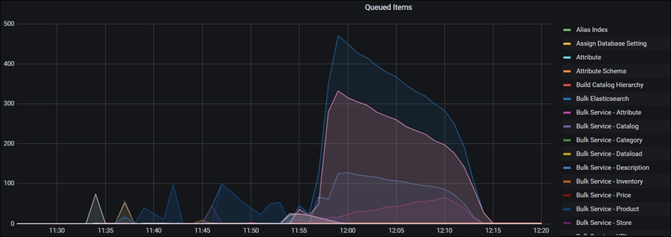
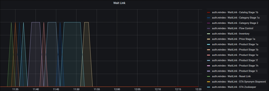
You can use Grafana to analyze the performance of the ingest pipeline. The two most useful graphs are Queued Items and WaitLink.
Visual Representation of the NiFi activities
In the NiFi ingest connectors, WaitLink process groups are added between process groups to ensure that the previous stage is completed before the next stage is started. This way, subsequent stages will not use data that is currently being worked on in an unfinished process. In addition, this reduces the occurrence of different processes running at the same time, which can cause extreme spikes in resource requests for CPU, network, memory or disk I/O.
NiFi uses "flow files" to process data in batches. The number of documents included in a flow file is defined by the scroll.bucket.size property. Setting (scroll.bucket.size)=300, for example, would allow 300 catentryIds per flowfile if applied to the Product Update 1i processing segment.
Both WaitLink and Bucket.Size values can be tracked in Grafana. Observing the activities and quantities helps determine system behavior and aids in the detection of slow segments.
Interpreting the graphs and detecting a bottleneck
The "wait link" and "queued items" graphs showing data for the Bulk Service Processor, are key metrics for understanding the Ingest/Index build operation. Bulk Service Processor values are important since they indicate packages sent to the Elasticsearch cluster. This is because all of the flowfile backlogs are found only inside of the Bulk Service and not in other Extract and Transform phases from each stage.
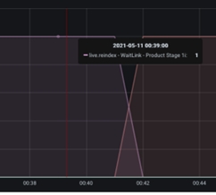
Both graphs have a number of metrics that can be tracked (by clicking the coloured line on the right side of the graph), but only the most key metrics are displayed by default. Hover the mouse pointer over the graph line and see which curve belongs to which process group or wait link. When the processor group name or wait link is clicked, a small pop-up box appears:
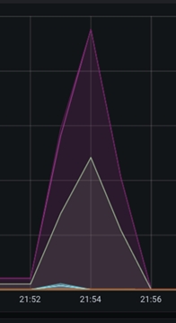
The "queued link" graph depicts the number of flow files queued for processing at a given processor group. A sharp rise in the curve indicates that the previous processor (or processor group) is processing data faster, or that the processor group is struggling to keep up with the overall throughput of adjacent processor groups. In the image below, you can observe a rapid increase in the number of queued items around the 21.54 timestamp, indicating that the processor is not keeping up with the incoming flow:
Similarly, the graph's ramp-down section has a steep curve, indicating that the CPU was able to complete the processing rapidly. The steeper the curve, the faster the processor can process the flowfiles, and the shallower the curve, the slower the processor can process the data. A case of sluggish data flow processing can be seen in the image below:
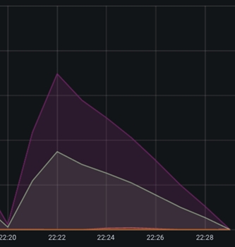
The incoming rate (centered at 22:22 timestamp) is substantially greater than the outgoing rate, with the incoming rate being relatively steep compared to the shallow angle of the outgoing curve.
These simple observations are simple to apply to graphs and identify potential bottlenecks. However, the conclusions are not always true, and the processor groups are sometimes constrained in their data processing. To conclude, more observations are needed to confirm the bottleneck.
Below the queued items are graphs of WaitLink. WaitLink graphs, unlike queued items, show which stage or segment is processing at any given time. In other words, while the X axis indicates time (corresponding to the Queue Item graph), the Y - axis shows the active segment, having values ranging from 0 to 1:
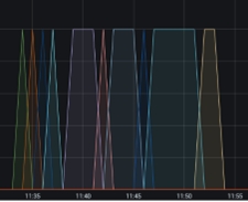
If the system supports various languages, you may see many WaitLinks appear at the same time. Thus, graphs reaching the Y axis up to value 2 may be shown for two languages, and so on.
Wait links are helpful in assessing which processing stage takes the longest to complete. The slowest segments are the longest rectangles, which are the best candidates for ingestion process optimization.
In the next topic let us explore few typical cases of suboptimal ingestion processing and you will formulate a strategy to improve the processing speed.