Advanced analytics
Advanced analytics functions provide specialized methods of analyzing time series data for patterns or abnormalities.
You use advanced analytics functions to perform the following types of analysis:
- Search based on specific measures like similarity, distance, and correlation. Find the portions of a sequence which are related to a given pattern.
- Quantify similarity, distance, and correlation between two sequences using the Lp-norm, Dynamic Time Warping, or Longest Common Subsequence method.
- Detect anomalies within time series data.
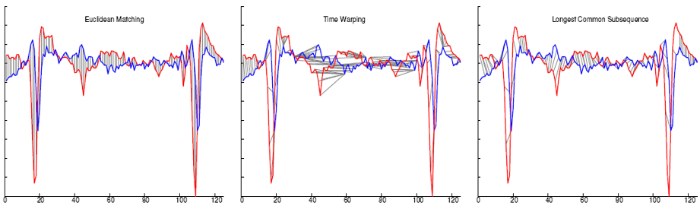
The following illustration shows different methods of comparing the same sequences. The Euclidean distance method, or the L2-norm method, does not find a match. Both the dynamic time warping and the longest common subsequence methods detect matches.
Lp-norm
The Lp-norm method measures the linear distance between two patterns. The Lp-norm method has the following characteristics:
- One-to-one comparisons of sequences
- Sequences must have equal length
- Results can be indexed in multi-dimensional indexes
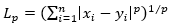
The standard Euclidean distance is expressed as L2-norm, where the value of p is 2 in the following formula:
Dynamic time warping
Dynamic time warping (DTW) is an algorithm for measuring similarity between two time-based sequences where the frequency of the observations is not synchronized between the two sequences. You can apply the DTW algorithm to linear numerical sequences of data, such as video, audio, and graphics data. The DTW algorithm calculates an optimal match between two given sequences with the sequences warped non-linearly in the time dimension to determine a measure of their similarity independent of certain non-linear variations in the time dimension.
DTW has the following characteristics:
- One-to-many mapping on sequence points
- Sequences are not required to have equal lengths
- Tolerance for noise so that two sequences can be similar even if a small part of the sequences are significantly divergent
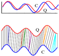
For an input time series of C1, C2, ..., Ci, and a pattern sequence of Q1, Q2, ..., Qj, the DTW score is computed with the following formula:
D(i,j)=|Ci – Qj|+min{D(i – 1,j),D(i – 1,j – 1),D(i,j – 1)}The score can be visualized as a mapping between C and Q.
You can constrain the DTW algorithm in the following ways:
- Sakoe-Chiba constraint
- The Sakoe-Chiba constraint forms a band to constrain the scoring. For an input time series of
C1, C2, ..., Ci, and a pattern sequence of Q1, Q2, ..., Qj, the DTW score with a Sakoe-Chiba
constraint is computed with the following
formula:
D(i,j)=|Ci – Qj|+min{D(i – 1,j),D(i – 1,j – 1),D(i,j – 1)},
      where  |i-j| < norm_mconstraint *  min(lengthof(C),lengthof(Q))
The following illustration shows how the Sakoe-Chiba constraint forms a band where the DTW score is computed.
Figure 4: C | Q mapping with an mConstraint 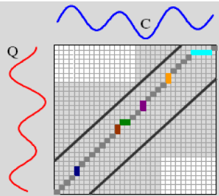
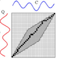
- Itakura Parallelogram constraint
- The Itakura Parallelogram constraint forms a parallelogram-shaped region where the DTW score is
computed, as shown in the following illustration.
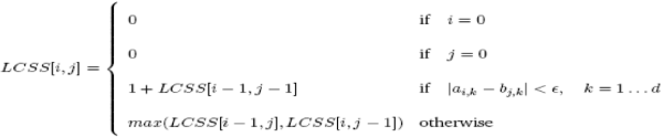
Longest common subsequence
The Longest common subsequence (LCSS) measures the similarity between two time series sequences.
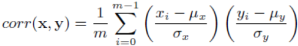
Pearson correlation coefficient
The Pearson correlation measures the degree of linear interrelation between two time series sequences. The Pearson correlation coefficient is obtained by dividing the covariance of the two variables by the product of their standard deviations. A correlation coefficient of 1 indicates an exact match.
Abnormal sequence detection
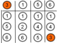
Abnormal sequence detection compares sequences to identify any sequences that are abnormal compared to other sequences. Given a long time series sequence, abnormal sequence detection provides the ability to tell which part of the time series is significantly different from the portion of data nearby in time order. For example, the tallest sequence in the following illustration is abnormal compared to the other sequences.
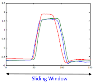
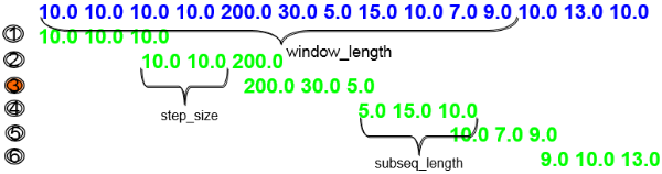
You specify a sliding window length, the size of the step to move the comparison, and the size of the sequence. This method checks how many neighbors of a sequence's top-k nearest neighbor sequences also consider the sequence as a top-k nearest neighbor.
For sequence 3, only its neighboring sequence 6 regards it as a top-3 neighbor, which implies that sequence 3 is a relative outlier in the set of sequences 1 - 6.